How to Code a Reinforcement Learning Model
Welcome back, fellow coders. In my last article, I discussed reinforcement learning, how it works, and the general use cases to get you familiar with it. Today we will look at an example illustrated by a car and a mountain. This example comes from a place you should never go, the 10th page of Google. Made in 2019, this monstrosity was no longer functional, but with a little (lot of) tweaking here and there, I was able to bring it to you today as a functional github repo. Today, we will teach an AI how to use momentum to climb a mountain.
Tutorial:
We are using Reinforcement Learning for this example. We feed the states and rewards to the RL agent and we get actions back.
First start by pip installing numpy and gymnasium in your terminal so that you can use the modules needed for this tutorial. We will use the numpy module for our data structure and to speed our code up and use gymnasium for our ai logic.
For any project you are going to want to import relevant modules. Modules have functions which you can use throughout your code and are extremely fast, which makes them great for your coding projects.
For this project we are going to use gymnasium for our ai logic and numpy for its impressive speed. At the top of your code type To start import gymnasium as gym and numpy as np at the top of our code so that we can use the module’s functions.
import gymnasium as gym
import numpy as np
Here we are making the environment that the ai will interact with.
Using the make function from the gymnasium module, let’s create the simulation and call it `env`. We’ll set the environment(env) to MountainCar, which is a preset created by OpenAI for us to experiment with, and the render mode to human so that it renders what’s happening in real time in a visual format.
# Create the MountainCar environment
env = gym.make(“MountainCar-v0”, render_mode=”human”)
We need an AI for this as it isn’t just moving forward. To make it up the mountain, the AI must figure out how but not just that it must go through a long process of trial and error. If the AI just does the +1 in this example, it doesn’t maximize the points whilst if it did the bottom route it would have turned out better and gotten a higher reward. That is why we should include an exploration and discount rate.
Let’s set the parameters for the learning rate, discount factor and epsilon/exploration rate, which is a measure of how adventurous it is. These parameters are often tweaked a lot when it comes to large-scale learning models. You can experiment with these values, see what is fastest and learn what the impact of each number is.
# Hyperparameters
learning_rate = 0.001
discount_factor = 0.1
epsilon = 0.2 # Exploration rate
Now let’s initialize settings for the q-table. We are essentially creating a list of lists expressed by the figure above. You can experiment with the discrete OS size variable by making it larger like [40,40] or smaller [4,4] or a lot bigger [1000, 1000]. Remember to be careful as depending on your computer, if it’s too large, you won’t be able to run your code. Generally you want these numbers to be divisible by four because they are easier to work with but for this project it shouldn’t matter too much.
# Discretization settings (similar to bucketing)
DISCRETE_OS_SIZE = [20, 20] #Initialize Parameters for q-learning
discrete_os_win_size = (env.observation_space.high — env.observation_space.low) / DISCRETE_OS_SIZE #
For this, we are using Q-tables, which is one of the three methods I discussed in my previous article [link].
Essentially, we are creating a multidimensional array of values, see figure 2, for how this looks. Using the values from the snippet above, we are generating a q-table. We are using numpy’s random uniform function and telling it to give us a list of random values from a min of -2 and a max of 0. Then we set the size to the variables we set earlier.
# Q-table initialized to random values between -2 and 0
q_table = np.random.uniform(low=-2, high=0, size=(DISCRETE_OS_SIZE + [env.action_space.n]))
By using the int32 function from numpy, we are dropping the decimal(32.9 → 32) then storing it using the astype function to speed the code up. After doing that, we return the value in a tuple which is the number format we are using for the coordinates. The function takes the current state as input, then uses that information to get the current position of the car and then returns it.
# Discretize the continuous state into a bucket index
def get_discrete_state(state):
discrete_state = (state - env.observation_space.low) / discrete_os_win_size
return tuple(discrete_state.astype(np.int32))
Here we are resetting the environment. This is to make sure we aren’t starting at where the car finished but the start. To do this, we are going to set the state and environment to 0/default settings.
# Reset environment and get initial discrete state
discrete_state = get_discrete_state(env.reset()[0]) # reset() returns a tuple, access
Define done which we will use for our while loop. We will be using this for a while loop. When we set done as True, we will stop our code.
done = FalseLet’s create the while loop. Essentially, this will run as long as done is set to False. This is pretty intuitive as Python is a readable language. While not done, repeat the process.
while not done:Here we are implementing the logic for the AI deciding whether to exploit or explore. If it chooses to exploit, it will use its pre-existing knowledge to make what it thinks is the best action. If it chooses to explore, it will choose a random action and based on that action
# Exploration vs. exploitation
if np.random.random() > epsilon:
# Exploit: choose action with the highest Q-value
action = np.argmax(q_table[discrete_state])
else:
# Explore: choose a random action
action = np.random.randint(0, env.action_space.n)
The dash is a placeholder for the values we don’t need for this example. State is the action the AI will take. Done is a boolean (True/False) value that we use to determine whether we should end the simulation
# Step the environment
new_state, reward, done, _, _= env.step(action)
Let’s now call the function we made and set the new_state to the value returned
new_discrete_state = get_discrete_state(new_state)Now, let’s get the position of the flag, which is where we want to incentivise the AI to go.
goal_position = env.unwrapped.goal_positionLet’s add if statements to check if the car made it to the goal or if the environment started the car at the goal instead of the place where it should be. Here we are going to put pass as a placeholder.
if not done:
  pass
elif new_state[0] >= env.goal_position:
  pass
Here we are going to update the q-table if the code isn’t done. Using np.max we will get the max future q table and the current by plugging our action. Now we will set the new_q table using learning_rate to determine the action multiplied by the current q. Then adding learning rate multiplied by the sum of the reward and quotient of the discount factor and max future q table.
if not done:
  # Update Q-table using Q-learning algorithm
  max_future_q = np.max(q_table[new_discrete_state])
  current_q = q_table[discrete_state + (action,)]
  new_q = (1 — learning_rate) * current_q + learning_rate * (reward + discount_factor * max_future_q)
  q_table[discrete_state + (action,)] = new_q
Now let’s add the logic for if the car spawns in at the end goal. Essentially we are resetting everything.
elif new_state[0] >= env.goal_position:
  # Reached the goal: reward is 0, set Q-value to 0
  q_table[discrete_state + (action,)] = 0
Let’s update the discretion state to the updated version.
# Move to the next state
discrete_state = new_discrete_state
Update the environment image.
  # Render the environment
  env.render()
Now let’s put this at the end of the while loop so once the while loop ends then this happens
env.close()Bonus:
Try to add a gradual decrease in the epsilon. You can try multiple different methods. The most common is this:
epsilon = epsilon * 0.99999999If you want to try an alternative path than try this. Here we are setting an exploration rate to be extremely high so that it gets a massive sample dataset and then from there makes decisions based on it:
# Hyperparameters
learning_rate = 0.001
discount_factor = 0.1
epsilon = 10000000000 # Exploration rate
And then add this to the top of your while loop
while not done:
  epsilon = epsilon * 0.90 if epsilon > 0.1 else epsilon
Instead of resetting each time it will save the data. To do this add
To save time and avoid resetting the environment each time, you can log the progress of your Q-table to a CSV file. This way, the AI will not have to start from scratch every time you stop the program. It’s also useful for tracking how well your AI is learning over time.
Step 1: Import the CSV module:
You’ll need to import the csv module at the beginning of your code so you can write the Q-table data to a file. If you don’t have it pip installed once again open your terminal and type `pip install csv`
import csvStep 2: Saving and Loading our Data
At the end of our code we will want to save the data to make the next time we run the simulation much faster as it is currently way too slow and forgets everything it learns.
First let’s start with the save_q_table function. To save the q-table we need values. The filename and updated q_table we are saving.
def save_q_table(q_table, filename):Introducing the `with` function if you haven’t heard of it. Essentially we are opening the file in a more secure way then typing open() close(). The mode is w for write and newline is for formatting and readability. The open tag gets the inputs we will use and then we set the value to the output as file. For csv files we need to first pass the info to a writer function so that we can write to it. Now we are going to write the new updated q values.
with open(filename, mode=’w’, newline=’’) as file:
  writer = csv.writer(file)
  for row in q_table:
    writer.writerow(row)
Now let’s add the load function to get the updated Q-table values and set them as our Q-table. Here we are going to use the reader function from the csv module to format our data. Then we are going to loop through the data that’s from the csv file and append/add a new list inside our list for every row there is.
def load_q_table(filename):
  q_table = []
  with open(filename, mode=’r’) as file:
    reader = csv.reader(file)
    for row in reader:
      q_table.append([float(value) for value in row])
  return q_table
Step 3:
At the start of our code let’s load in the previous q table and set it to our q-table.
q_table = load_q_table(‘final_q_table.csv’)But there’s an error. Instead add a try and except block so that if the file exists we use it and if it doesn’t we append our new file to it.
try:
  q_table = load_q_table(‘final_q_table.csv’)
except:
  q_table = np.random.uniform(low=-2, high=0, size=(DISCRETE_OS_SIZE + [env.action_space.n]))#
Step 4:
At the end of your code call your function and give it the new updated q-table and if you want to get fancy you can add a print statement just before it.
save_q_table(q_table, ‘final_q_table.csv’)How I started
Since I was little, I was always interested in AI. That is why today I started my Reinforcement Learning Journey at TKS. I decided to start with a Reinforcement Learning tutorial, totally oblivious to the date/how outdated the module was and sure enough, when it came for me to run the code, it didn’t work. Here is where the challenges arose, but despite the challenges I continued. I found more recent modules and adjusted the code accordingly.
My process
To start I imported the gymnasium and numpy modules for this project. Then I created the MountainCar environment using the gymnasium module. Next I decided to go with a learning rate of 0.01, a discount factor of 5.0, and an epsilon of 10 which is a fancy way of saying Exploration rate. Then I followed the tutorial with a few minor adjustments until I got another error and modified the discrete state, which resets the environment and got an initial discrete state, which resets the environment and returns a tuple, and accesses the first element. It was working fine until it reached the point where I updated the q-table. Once again I had to debug and fix the code. The step function wasn’t working anymore so I did some research and I figured out that the notation had changed along with a new API being introduced. This was the final error and I finally was left with a classic momentum RL implementation.


